Excel Error Codes Explained: What Each One Means

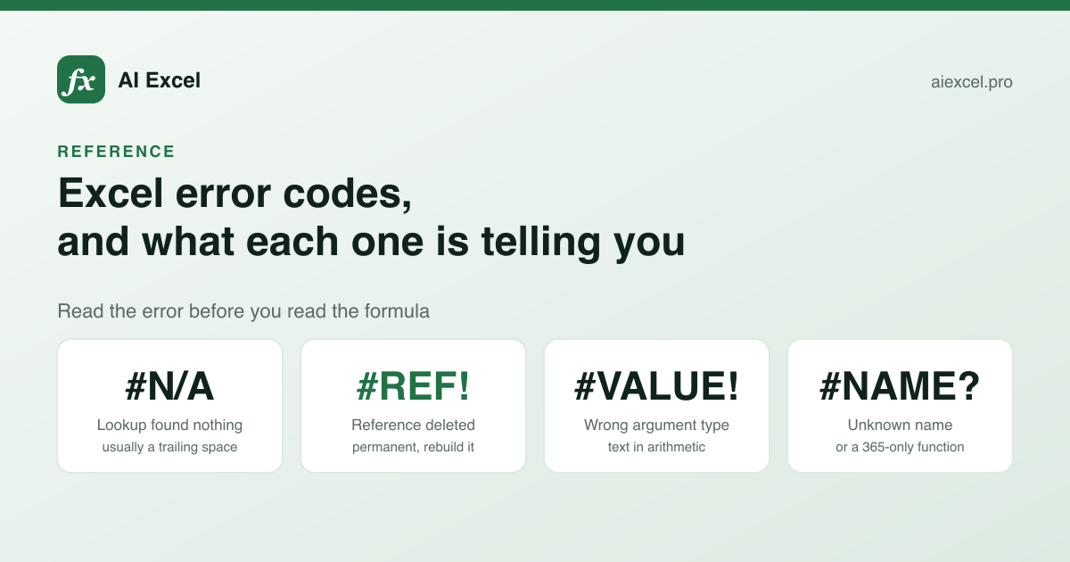
Excel has nine error values, and each one narrows the cause enormously before you read a single character of the formula. #N/A and #VALUE! are not two flavours of "something went wrong" — they point at different mistakes and want different fixes.

This is what each one means, the cause behind it most of the time, and how to fix it without hiding it.

Start here

#N/A — the lookup found nothing

This is the most common error and the most commonly misdiagnosed, because it is usually not a missing value. The value is there; something about it does not match.

The four causes, in order of frequency:

• Trailing whitespace. Data exported from another system is full of it, and it is invisible. TRIM() both sides.
• Text versus number. The ID is 1042 in one column and "1042" in the other. They look identical. ISNUMBER() on both tells you in a second.
• Approximate match on unsorted data. VLOOKUP's fourth argument defaults to TRUE. Pass FALSE.
• The lookup range does not extend far enough. A range ending at row 500 in a table that now has 800.

=IFERROR(VLOOKUP(F2,A:C,3,FALSE),"")

// Also swallows #REF! from a deleted
// column, and #NAME? from a typo.
// The sheet looks fine and is wrong.

=IFNA(VLOOKUP(F2,A:C,3,FALSE),"")

// #N/A becomes blank.
// #REF! still shows as #REF!,
// which is what you want.

#REF! — something it pointed at is gone

The reference itself was destroyed, usually by deleting a column or row that a formula depended on. Unlike most errors this one is permanent: the formula literally now contains the text #REF! where the reference used to be, so undoing the deletion afterwards does not restore it.

If you catch it immediately, Ctrl+Z is the fix. If you do not, the formula has to be rebuilt. This is the strongest practical argument for INDEX/MATCH over VLOOKUP — INDEX references a column rather than counting to it, so it survives inserts, and it fails loudly rather than quietly returning the wrong column.

#VALUE! — the wrong kind of thing

A function got an argument of a type it cannot use. Most often that is arithmetic touching a cell containing text — including text that looks like a number, and including a cell that contains a single space and therefore is not empty.

The other common cause is handing a range to something that wanted one cell. Older Excel does this constantly; newer Excel often spills instead, which can be a surprise of its own.

To diagnose: =ISNUMBER(A2) on the cells feeding the formula. One of them will be FALSE and that is your answer. VALUE() converts clean text digits; NUMBERVALUE() handles the case where the separators are from another locale.

#DIV/0! — usually blank, not zero

An empty denominator cell evaluates to zero, so this fires on missing data as readily as on an actual zero. The distinction matters for the fix: if the denominator is legitimately zero, showing a dash is correct; if it is missing, showing a dash hides a data problem.

// Hides both cases identically
=IFERROR(B2/C2, "-")

// Distinguishes them
=IF(C2="", "no data", IF(C2=0, "-", B2/C2))

#NAME? — Excel does not know that word

Three causes. A misspelled function name. A named range that does not exist, or was deleted. Or — the one that catches people out — a function that exists in your Excel and not in theirs.

A workbook using XLOOKUP, LET or TEXTSPLIT opens as #NAME? on Excel 2019 with no explanation. If a formula works for you and errors for a colleague, check the function's availability before checking anything else — every page in the function reference states which versions support it.

Text missing its quotes produces this too: =IF(A2=West,1,0) asks Excel for a named range called West.

#SPILL! — the newest one

Dynamic array formulas write into the cells below and to the right of themselves. If any of those cells is occupied — including by a space, or by a merged cell — the formula cannot spill and returns #SPILL!.

Excel highlights the blocked range when you select the cell, which makes this one of the easier errors to fix. Merged cells in the spill zone are the cause people miss, because the blocking cell looks empty.

#NUM! and #NULL!

#NUM! means the calculation is impossible or did not converge: the square root of a negative, a date before 1 January 1900, or IRR failing to find a rate. For the iterative financial functions, supplying a sensible guess argument often fixes it.

#NULL! is the rarest. It means you used the intersection operator — a space — between two ranges that do not overlap. In practice it is always a typo where a comma was intended.

Finding the error in a long formula

The rule about IFERROR

Use IFERROR only where you have decided that every possible error is acceptable. That is a much rarer situation than its usage suggests.

For a lookup that may legitimately miss, use IFNA. For division, test the denominator. For a whole column wrapped in IFERROR "to clean it up", assume there is a real error in there somewhere and go looking before you ship it.

If you have a formula erroring and cannot see why, paste it into the formula explainer along with the error code you are seeing — the explanation focuses on what in that formula produces that specific error.